pass@k

Definition

pass@k measures the probability of finding at least one correct solution within a random sample of $k$ solutions, drawn from a larger pool of $n$ independently generated attempts.

Formula

let $D=\{q_i,a_i{\}}_{i=1}^{i=m}$ be a test dataset

• of size $m$,
• with questions $q_i$,
• and answers $a_i$,

let $D_G=\{q_i,\{{\hat{a}}_{ij}{\}}_{j=1}^{j=n}{\}}_{i=1}^{i=m}$ be a dataset of independently generated answers where

• $n$ is the number of generated answers per question,
• ${\hat{a}}_{ij}$ is the model’s 𝑗-th final answer for $q_i$,
• $c_i$ is the number of correct solutions for $q_i$ in $\{{\hat{a}}_{ij}{\}}_{j=1}^{j=n}$

then

$$pass@k=1-{\mathbb{E}}_{D_G}\left[\frac{\left(\genfrac{}{}{0ex}{}{n-c}{k}\right)}{\left(\genfrac{}{}{0ex}{}{n}{k}\right)}\right]$$

let’s break this formula step-by-step:

• $\left(\genfrac{}{}{0ex}{}{n-c}{k}\right)$ computes the number of combination of $k$ incorrect samples
• $\left(\genfrac{}{}{0ex}{}{n}{k}\right)$ computes the number of total combination of $k$ samples
• $\frac{\left(\genfrac{}{}{0ex}{}{n-c}{k}\right)}{\left(\genfrac{}{}{0ex}{}{n}{k}\right)}$ computes the probability of drawing only incorrect samples
• $1-\left[\frac{\left(\genfrac{}{}{0ex}{}{n-c}{k}\right)}{\left(\genfrac{}{}{0ex}{}{n}{k}\right)}\right]$ computes the inverse event, which is drawing at least one correct sample.

Example

Let’s get through a simple example of a dataset of size $m=1$. For a real dataset, all individual $pass@k$ are averaged across all samples.

Imagine a language model is tasked with writing a Python function to check if a number is prime. To evaluate its performance on this task, we generate 200 code samples ($n=200$). After running unit tests on all of them, we find that 10 of the samples are correct ($c=10$).

Now, let’s calculate $pass@1$, $pass@5$, and $pass@10$.

Calculating $pass@1$:

This tells us the probability that a single, randomly chosen sample is correct.

Using the formula:

$$\begin{array}{rl}pass@1& =1-\left[\frac{\left(\genfrac{}{}{0ex}{}{200-10}{1}\right)}{\left(\genfrac{}{}{0ex}{}{200}{1}\right)}\right]\\ & =1-\left[\frac{190}{200}\right]\\ & =1-0.95\\ & =0.05\end{array}$$

So, there is a 5% chance that any single generated sample is correct. This is identical to $pas{s}^1$.

Calculating $pass@5$:

This is the probability that at least one of 5 randomly chosen samples is correct.

Using the formula:

$$\begin{array}{rl}pass@5& =1-\left[\frac{\left(\genfrac{}{}{0ex}{}{200-10}{5}\right)}{\left(\genfrac{}{}{0ex}{}{200}{5}\right)}\right]\\ & =1-\left[\frac{\frac{190!}{5!\times 185!}}{\frac{200!}{5!\times 195!}}\right]\\ & =1-\left[\frac{190\times 189\times 188\times 187\times 186}{200\times 199\times 198\times 197\times 196}\right]\\ & \approx 1-0.77\\ & \approx 0.23\end{array}$$

So, there is approximately a 23% chance of finding a correct solution within the top 5 generated samples.

Calculating $pass@10$:

This is the probability that at least one of 10 randomly chosen samples is correct.

The calculation would continue in the same manner:

$$\begin{array}{rl}pass@10& =1-\left[\frac{\left(\genfrac{}{}{0ex}{}{200-10}{10}\right)}{\left(\genfrac{}{}{0ex}{}{200}{10}\right)}\right]\end{array}$$

The resulting value will be higher than $pass@5$, indicating an increased likelihood of finding a correct solution as we consider more samples.

Usage

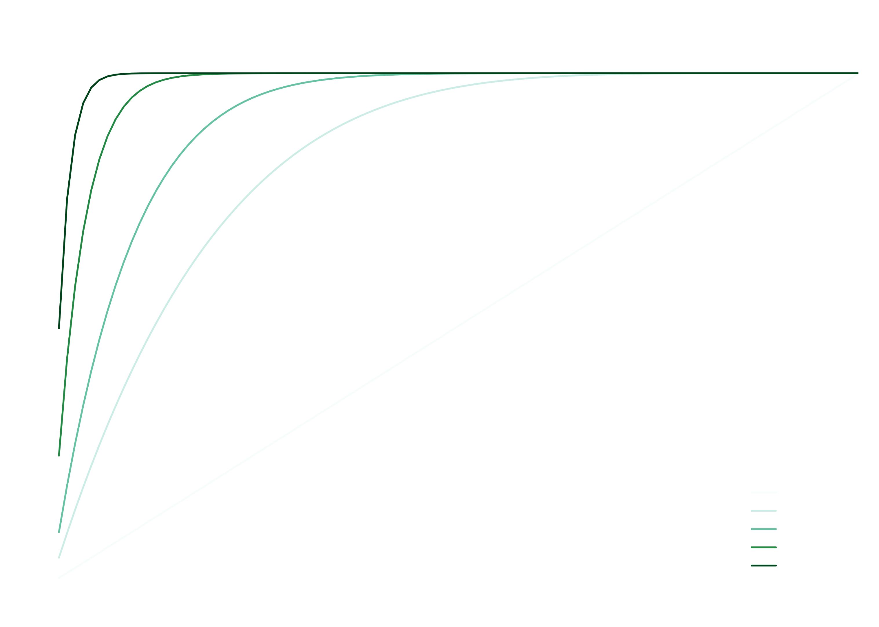
• $pass@k$ can be misleading as it may inflate a model’s perceived performance. The metric focuses on the probability of finding at least one correct solution within $k$ attempts, which can mask a low rate of first-try success. As the plot below illustrates, the $pass@k$ value often rises sharply with $k$.
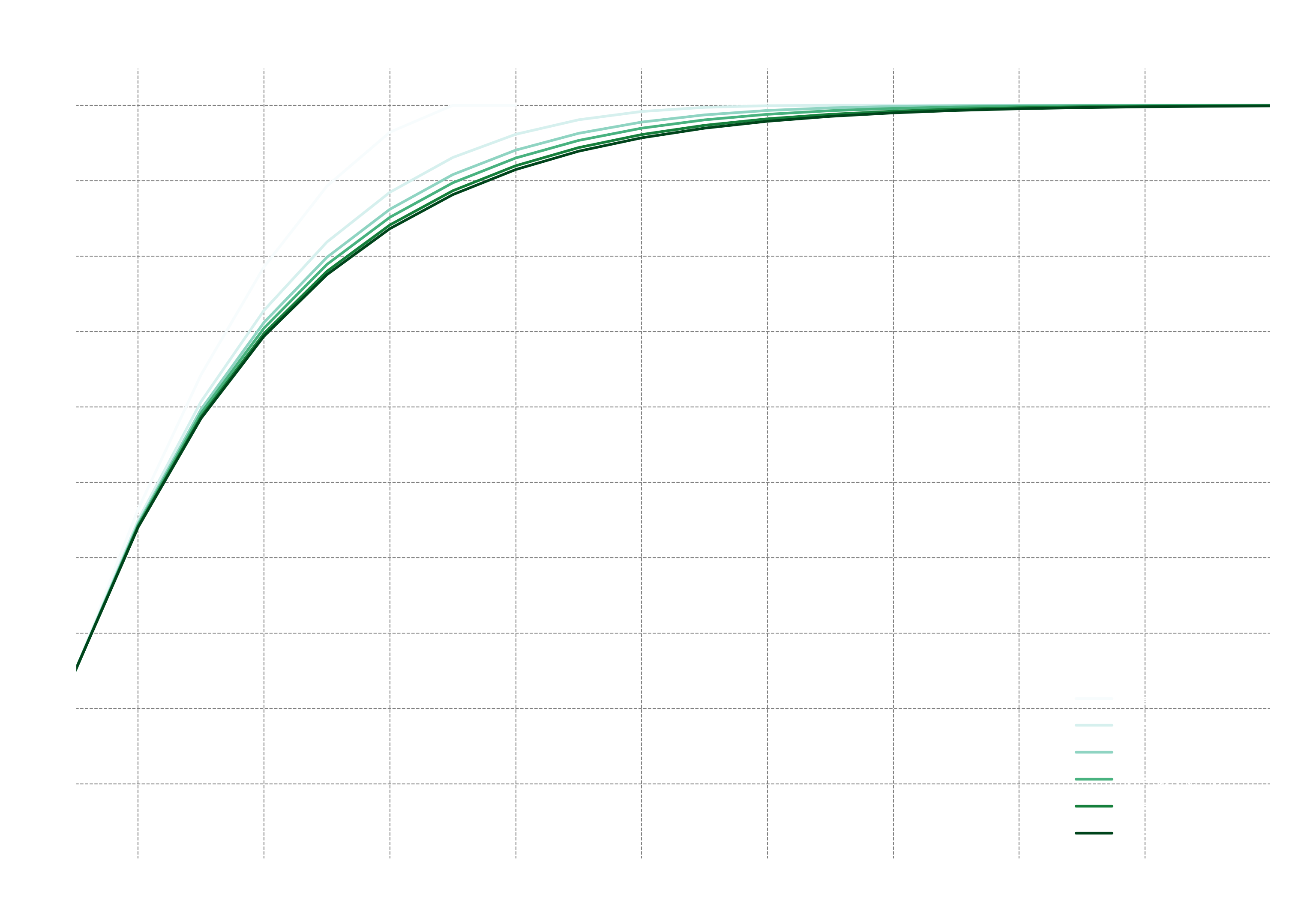
• Although the sample size ($n$) is not part of the metric’s name, it is a critical factor in its interpretation. For a fixed success rate, a larger sample size ($n$) provides a more rigorous evaluation and results in a more conservative (i.e., lower) $pass@k$ score.
• The $pass@k$ metric is most suitable for tasks where solutions can be verified automatically and inexpensively. A prime example is code generation, where unit tests can validate solutions without human intervention. In such scenarios, $pass@k$ serves as an excellent measure of a model’s practical utility—the likelihood it will provide a working solution within a few attempts.