Effect of the initial configuration of weights on the training and function of artificial neural networks

Abstract

The function and performance of neural networks is largely determined by the evolution of their weights and biases in the process of training, starting from the initial configuration of these parameters to one of the local minima of the loss function. We perform the quantitative statistical characterization of the deviation of the weights of two-hidden-layer ReLU networks of various sizes trained via Stochastic Gradient Descent (SGD) from their initial random configuration. We compare the evolution of the distribution function of this deviation with the evolution of the loss during training.

Key takeaways

• Successful training via SGD leaves the network in the close neighborhood of the initial configuration of its weights.
• An abrupt increase of the distribution function of the deviation from initial weight to current value within the overfitting region. This jump occurs simultaneously with a similarly abrupt increase recorded in the evolution of the loss function. This sharp increase closely correlates with the crossover between two regimes of the network—trainability and untrainability.
• SGD’s ability to efficiently find local minima is restricted to the vicinity of the random initial configuration of weights.
• In order to reach an arbitrarily chosen loss value, the weights of larger networks tend to deviate less from their initial values (on average) than the weights of smaller networks.
• Weights that start with larger absolute values are more likely to suffer larger updates (in the direction that their sign points to).
• The success of training highly over-parameterized networks may be due to their initial random configuration being close to a suitable minimum. Reaching this minimum requires only slight adjustments to the weights, leaving recognizable traces of the initial configuration.

Experiment

Preliminary concepts

• Glorot’s uniform initialization :

$w_{ij}\sim U\left(-\frac{\sqrt{6}}{\sqrt{m+n}},\frac{\sqrt{6}}{\sqrt{m+n}}\right)$

where ($U(-x,x)$ represents the uniform distribution within the interval (-x, x), m and n are the number of units in the layers connected by $w_{ij}$.)

Objectives

• Characterize how much the weights of a neural network deviate from their initial random configuration during training.
• Explore the relationship between the initial configuration of weights and the success of the training process.
• Investigate the phenomenon of a neural network crossing over between regimes of trainability and untrainability.
• Explore the connection between network trainability and the distance a network travels from its initial configuration of weights.

Setup

• Feedforward neural networks : 2 ReLU(hidden layers), each containing 10 to 1000 units + output layer using softmax. This architecture is similar to a Keras-created multilayer perceptron for MNIST.
• Glorot initialization.
• 3 datasets: MNIST, Fashion MNIST, and HASYv2.
• Loss : categorical cross-entropy
• SGD (learning_rate = 0.1, batch_size=128)
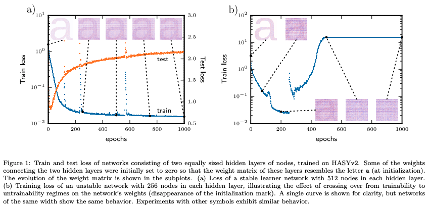
• to illustrate the reduced scale of the deviations of weights during the training, network’s initial configuration of weights has been marked using a mask in the shape of a letter (Fig. 1)

Results

• Figure 1(a) showcases a large network (512 nodes in each hidden layer) where some initial weights were set to zero to create a visual mark resembling the letter “a”. After training for 1000 epochs, the mark remains clearly visible, indicating that the weights have not significantly deviated from their initial values. This supports the observation that larger networks tend to stay close to their initialization during training.
• In contrast, Figure 1(b) depicts an unstable, mid-sized network (256 nodes per hidden layer) where the initial “a” marking disappears during training. The significant changes in weights coincide with the network’s transition to the untrainability regime, marked by a sharp increase in the training loss. This observation suggests that unstable networks undergo substantial weight changes as they cross over from trainability to untrainability.

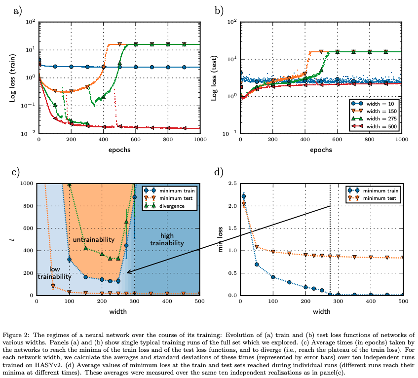
• Figure 2(a) and 2(b) depict the evolution of training and test loss functions, respectively, for networks with varying widths. The plots illustrate the three training regimes: high trainability (low loss, small deviations), low trainability (higher loss, larger deviations), and untrainability (loss increase, large deviations). Wider networks (strong learners) exhibit high trainability, while smaller networks (weak learners) struggle to achieve low losses. Unstable learners initially show a decrease in loss but eventually diverge.

• Figure 2(c) presents a “phase diagram” that maps the network’s training regime based on its width and training time. The diagram showcases the transition points for minimum training loss, minimum test loss, and divergence (sharp loss increase). Wider networks tend to remain in the high trainability regime, while narrower networks often transition to untrainability.

• Figure 2(d) displays the average minimum loss values attained during training and testing for networks of different widths. Wider networks achieve lower minimum losses, indicating better trainability.

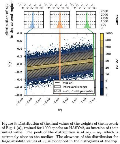
• Figure 3 analyzes the distribution of final weight values ($w_f$) after training with respect to their initial values ($w_i$) for the stable network shown in Figure 1(a). The peak of the distribution lies near the line $w_f=w_i$, signifying minimal weight changes during training. However, the figure also shows a skew, with initially larger weights tending to increase further, suggesting that the learning process favors and amplifies weights that were already strong at initialization.